Analyze Bootstrap Experiment Results

Define Libraries

library("stringr")
library("dplyr")
library("reshape2")
library("ggplot2")

Define Path

dir.wrk <- str_replace(getwd(), "/scripts", "")
dir.output <- file.path(dir.wrk, "output")

Define Files

file.dat <- file.path(dir.output, "stats_anovatbl_permanova_permmute_results_withReplacement.tsv")

Load Data

dat <- read.delim(file.dat, header = TRUE, stringsAsFactors = FALSE)

Get R2 data for plotting

df <- subset(dat, dat$Category == "R2")
df$Category <- NULL
df <- subset(df, df$Feature %in% c("Ethnicity", "IncomeGroup", "EducationLevel", 
    "GeoRegion"))

# RESHAPE DATA ---
dm <- reshape2::melt(df, id.var = "Feature", value.name = "R2")
dm$Feature <- factor(dm$Feature, levels = c("Ethnicity", "IncomeGroup", "EducationLevel", 
    "GeoRegion"))

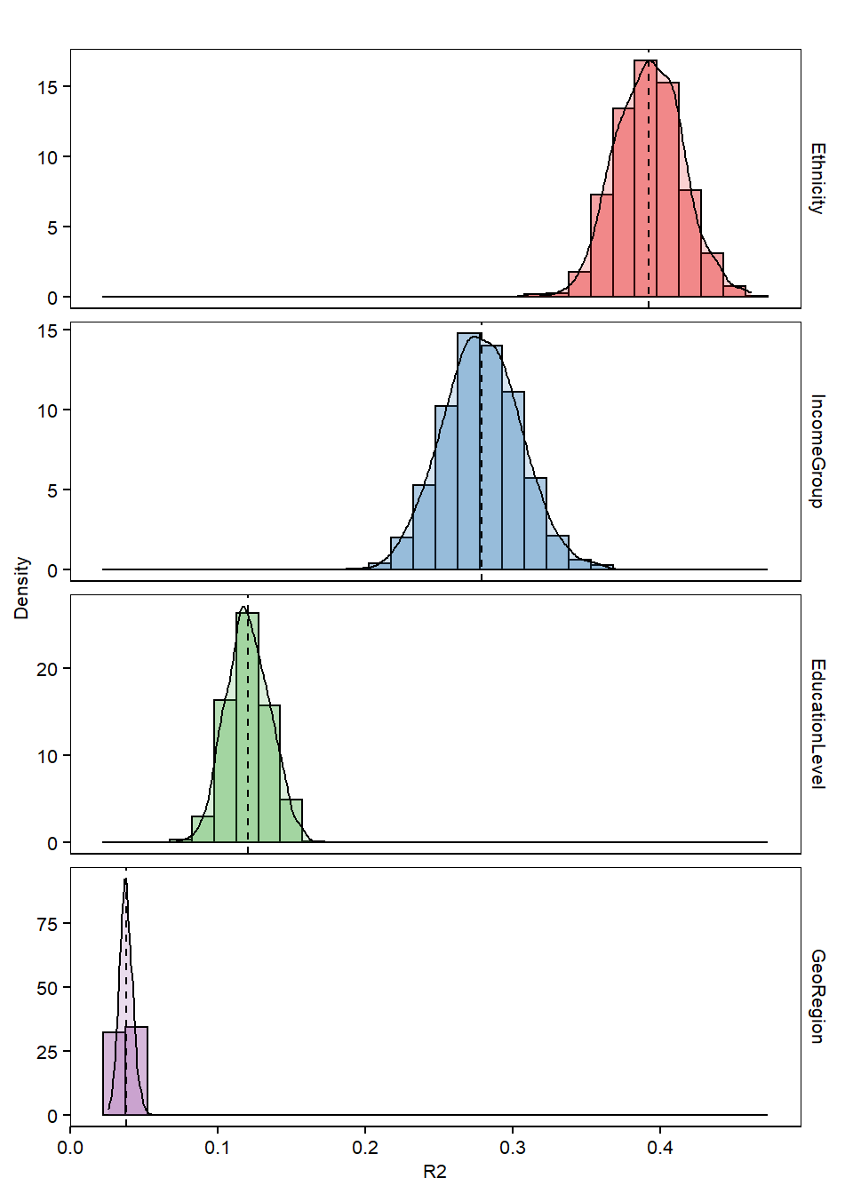
Mean and Standard Deviation of bootstrapped R2, grouped by different factors

summary_r2 <- dm %>% dplyr::group_by(Feature) %>% dplyr::summarise(mean = mean(R2), 
    std_dev = sd(R2))

summary_r2

## # A tibble: 4 x 3
##   Feature          mean std_dev
##   <fct>           <dbl>   <dbl>
## 1 Ethnicity      0.392  0.0225 
## 2 IncomeGroup    0.279  0.0261 
## 3 EducationLevel 0.121  0.0146 
## 4 GeoRegion      0.0379 0.00448

Plot Histogram of R2

# COLOR ---
cpalette <- c("#e41a1c","#377eb8","#4daf4a","#984ea3")
     
# PLOT ---
p <- ggplot(dm, aes(x=R2)) +
          geom_histogram(aes(fill=Feature, y=..density..), position="identity", color="#000000", alpha=0.4) +
          geom_density(aes(fill=Feature), alpha=0.2) +
          scale_fill_manual(values=cpalette) +
          geom_vline(data=summary_r2, aes(xintercept=mean), linetype="dashed", size=0.5, colour="#000000") +
          facet_wrap(~Feature, ncol=1, scales="free_y", strip.position="right") +
          theme(
               axis.text.x = element_text(size = 8, color="#000000"),
               axis.text.y = element_text(size = 8, color="#000000"),
               axis.title = element_text(size = 8, color="#000000"),
               plot.title = element_text(size = 10, color="#000000", hjust=0.5),
               panel.grid.major = element_blank(),
               panel.grid.minor = element_blank(),
               axis.ticks = element_line(size=0.4, color="#000000"),    
               strip.text = element_text(size=8, color="#000000"),
               strip.background = element_rect(fill="#FFFFFF", color="#FFFFFF"),
               panel.background = element_rect(fill="#FFFFFF", color="#000000"),
               legend.text = element_text(size = 10, color="#000000"),
               legend.title = element_blank(),
               legend.key.size = unit(0.5, "cm"),
               legend.position = "none") +
          ylab("Density") +
          xlab("R2") + 
          ggtitle("") 

p

## `stat_bin()` using `bins = 30`. Pick better value with `binwidth`.

Get Pvalue data

df <- subset(dat, dat$Category == "Pr..F.")
df$Category <- NULL
df <- subset(df, df$Feature %in% c("Ethnicity", "IncomeGroup", "EducationLevel", 
    "GeoRegion"))

# RESHAPE DATA ---
dm <- reshape2::melt(df, id.var = "Feature", value.name = "pvalue")
dm$Feature <- factor(dm$Feature, levels = c("Ethnicity", "IncomeGroup", "EducationLevel", 
    "GeoRegion"))

Mean and Standard Deviation of bootstrapped pvalue, grouped by different factors

summary_pvalue <- dm %>% dplyr::group_by(Feature) %>% dplyr::summarise(mean = mean(pvalue), 
    std_dev = sd(pvalue))

summary_pvalue

## # A tibble: 4 x 3
##   Feature         mean std_dev
##   <fct>          <dbl>   <dbl>
## 1 Ethnicity      0.001       0
## 2 IncomeGroup    0.001       0
## 3 EducationLevel 0.001       0
## 4 GeoRegion      0.001       0