Ordination Analysis
Define Libraries
library("stringr")
library("dplyr")
library("reshape2")
library("ggplot2")
library("RColorBrewer")
library("vegan")
Define Path
dir.wrk <- getwd()
dir.data <- file.path(dir.wrk, "data/data_household")
dir.annot <- file.path(dir.wrk, "data/data_annotations")
dir.output <- file.path(dir.wrk, "data/data_processed")
Define Files
file.dat <- file.path(dir.output, "household_level_data_frequency_table.tsv")Define Categories
type_eth <- c("Newar","Brahman","Madhesi","Chettri","Muslim−Others",
             "Gurung−Magar","Dalit","Rai−Limbu","Tamang","Chepang−Thami")
type_fuel <- c("Wood","LP Gas","Gobar Gas","Kerosene","Electricity","Others")
type_inc <- c("0-10000","10000-20000","20000-30000","30000-50000","50000-ABOVE")
type_edu <- c("Illiterate","NonFormal-Other","Primary","Secondary","University")
type_geo <- c("Himalayan","Hilly")

cpalette.eth <- c("#e31a1c","#a6cee3","#1f78b4","#b2df8a","#33a02c",
                  "#fb9a99","#fdbf6f","#ff7f00","#cab2d6","#6a3d9a")
cpalette.inc <- c("#fdd49e","#fdbb84","#fc8d59","#e34a33","#b30000")
cpalette.edu <- c("#bfd3e6","#9ebcda","#8c96c6","#8856a7","#810f7c")
cpalette.geo <- c("#35978f","#bf812d")
cpalette.grp <- c("#E31A1C","#BDBDBD")
Load Frequency Table Data
dat <- read.delim(file.dat, header=TRUE, stringsAsFactors=FALSE)
dat <- dat[-which(rowSums(dat[,5:10]) == 0),]

head(dat)
## Ethnicity EducationLevel GeoRegion IncomeGroup Electricity GobarGas Kerosene
## 1 Brahman Illiterate Hilly 0-10000 0 159 5
## 2 Brahman Illiterate Hilly 10000-20000 0 213 1
## 3 Brahman Illiterate Hilly 20000-30000 1 95 0
## 4 Brahman Illiterate Hilly 30000-50000 0 27 0
## 5 Brahman Illiterate Hilly 50000-ABOVE 0 9 0
## 6 Brahman Illiterate Himalayan 0-10000 1 24 1
## LPGas Others Wood
## 1 375 3 7932
## 2 666 1 3245
## 3 336 0 1038
## 4 109 0 355
## 5 69 1 156
## 6 118 4 5608Transform Data to log Scale
df <- vegan::decostand(dat[,5:10], "log")
df <- cbind(dat[,-c(5:10)], df)

df$Ethnicity <- factor(df$Ethnicity, levels=type_eth)
df$IncomeGroup <- factor(df$IncomeGroup, levels=type_inc)
df$EducationLevel <- factor(df$EducationLevel, levels=type_edu)
df$GeoRegion <- factor(df$GeoRegion, levels=type_geo)

head(df)
## Ethnicity EducationLevel GeoRegion IncomeGroup Electricity GobarGas Kerosene
## 1 Brahman Illiterate Hilly 0-10000 0 8.312883 3.321928
## 2 Brahman Illiterate Hilly 10000-20000 0 8.734710 1.000000
## 3 Brahman Illiterate Hilly 20000-30000 1 7.569856 0.000000
## 4 Brahman Illiterate Hilly 30000-50000 0 5.754888 0.000000
## 5 Brahman Illiterate Hilly 50000-ABOVE 0 4.169925 0.000000
## 6 Brahman Illiterate Himalayan 0-10000 1 5.584963 1.000000
## LPGas Others Wood
## 1 9.550747 2.584963 13.953469
## 2 10.379378 1.000000 12.664003
## 3 9.392317 0.000000 11.019591
## 4 7.768184 0.000000 9.471675
## 5 7.108524 1.000000 8.285402
## 6 7.882643 3.000000 13.453271Compute Distance Matrix
dm <- vegan::vegdist(x=as.matrix(df[,5:10]), method="euclidean",
                     binary=FALSE, diag=TRUE, upper=TRUE, na.rm=FALSE)
A. Ordination: by Ethnicity
# BETA DIVERSITY ---
bd_eth <- vegan::betadisper(d=dm, group=df$Ethnicity, type="centroid")

bd_eth
##
## Homogeneity of multivariate dispersions
##
## Call: vegan::betadisper(d = dm, group = df$Ethnicity, type =
## "centroid")
##
## No. of Positive Eigenvalues: 6
## No. of Negative Eigenvalues: 0
##
## Average distance to centroid:
## Newar Brahman Madhesi Chettri Muslim-Others
## 3.872 3.876 3.247 3.954 3.128
## Gurung-Magar Dalit Rai-Limbu Tamang Chepang-Thami
## 4.066 4.709 3.575 4.393 3.799
##
## Eigenvalues for PCoA axes:
## PCoA1 PCoA2 PCoA3 PCoA4 PCoA5 PCoA6
## 11684.2 1048.3 847.6 436.9 159.2 139.1# GET EIGENVALUES ---
d_eth <- data.frame(Ethnicity=df$Ethnicity, bd_eth$vectors[,1:2])
d_eth$Ethnicity <- factor(d_eth$Ethnicity, levels=type_eth)Plot Ordination
# PLOT ---
p1 <- ggplot(d_eth, aes(x=PCoA1, y=PCoA2)) +
          geom_hline(yintercept=0, linetype="dashed", color = "#bdbdbd") +
          geom_vline(xintercept=0, linetype="dashed", color = "#bdbdbd") +
          geom_point(aes(fill=Ethnicity, color=Ethnicity), size=3, shape=16) +
          scale_color_manual(values=cpalette.eth) +
          coord_cartesian(xlim=c(-11, 11), ylim=c(-5,5.2)) +
          theme(
               axis.text.x = element_text(size = 10, color="#000000"),
               axis.text.y = element_text(size = 10, color="#000000"),
               axis.title = element_text(size = 10, color="#000000"),
               plot.title = element_text(size = 15, color="#000000", hjust=0.5),
               panel.grid.major = element_blank(),
               panel.grid.minor = element_blank(),
               axis.ticks = element_line(size=0.4, color="#000000"),
               strip.text = element_text(size=10, color="#000000"),
               strip.background = element_rect(fill="#FFFFFF", color="#FFFFFF"),
               panel.background = element_rect(fill="#FFFFFF", color="#000000"),
               legend.text = element_text(size = 10, color="#000000"),
               legend.title = element_blank(),
               legend.key.size = unit(0.5, "cm"),
               legend.position = "right") +
          ylab("PCoA2") +
          xlab("PCoA1") +
          ggtitle("Ethnicity")

p1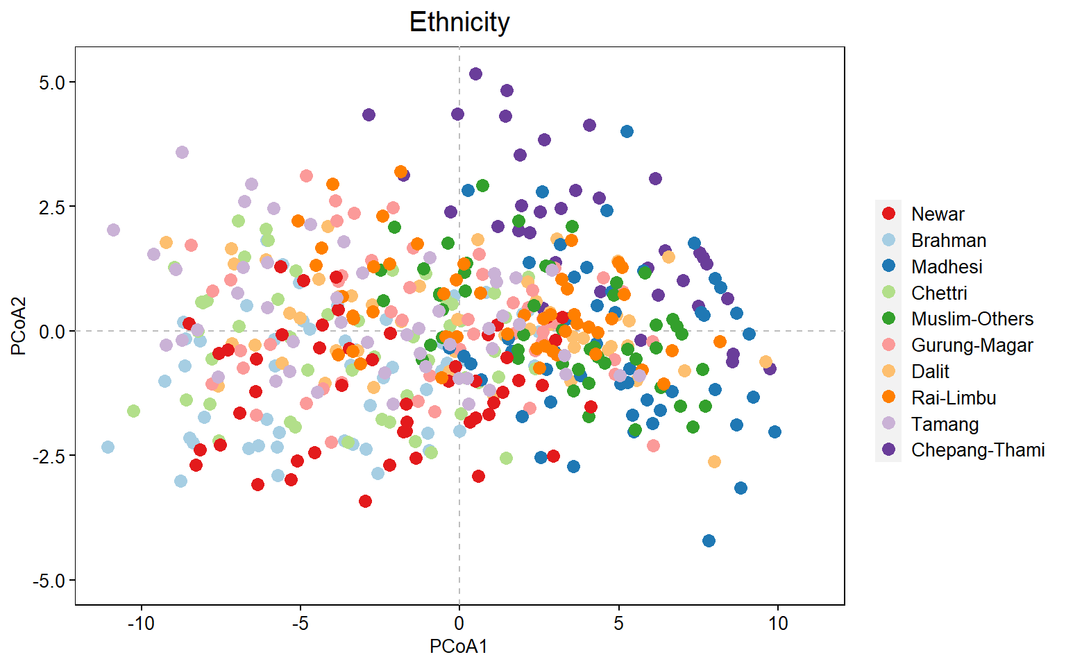
Prepare data for Segregated Plot by Ethnicity
# PREPARE DATA ---
list.dt <- list()
for(k in 1:length(type_eth)){
  d <- d_eth
  d$Label <- "bg"
  d$Group <- type_eth[k]
  ind <- which(str_detect(as.character(d$Ethnicity), type_eth[k]) == TRUE)
  d$Label[ind] <- "fg"
  d <- d[order(d$Label, decreasing = FALSE),]
  list.dt[[k]] <- d
}

# AGGREGATE DATA ---
dt <- do.call(rbind.data.frame, list.dt)

# FACTORIZE ---
dt$Ethnicity <- factor(dt$Ethnicity, levels=type_eth)
dt$Group <- factor(dt$Group, levels=type_eth)
dt$Label <- factor(dt$Label, levels=c("fg","bg"))
Plot Ordination
# PLOT ---
p11 <- ggplot(dt, aes(x=PCoA1, y=PCoA2)) +
          geom_hline(yintercept=0, linetype="dashed", color = "#bdbdbd") +
          geom_vline(xintercept=0, linetype="dashed", color = "#bdbdbd") +
          geom_point(aes(fill=Label, color=Label), size=2, shape=16) +
          scale_color_manual(values=cpalette.grp) +
          coord_cartesian(xlim=c(-11, 11), ylim=c(-5,5.2)) +
          facet_wrap(~Group, ncol=5, scales="fixed", drop=FALSE, strip.position="top") +
          theme(
               axis.text.x = element_text(size = 10, color="#000000"),
               axis.text.y = element_text(size = 10, color="#000000"),
               axis.title = element_text(size = 10, color="#000000"),
               plot.title = element_text(size = 15, color="#000000", hjust=0.5),
               panel.grid.major = element_blank(),
               panel.grid.minor = element_blank(),
               axis.ticks = element_line(size=0.4, color="#000000"),
               strip.text = element_text(size=10, color="#000000"),
               strip.background = element_rect(fill="#FFFFFF", color="#FFFFFF"),
               panel.background = element_rect(fill="#FFFFFF", color="#000000"),
               legend.text = element_text(size = 10, color="#000000"),
               legend.title = element_blank(),
               legend.key.size = unit(0.5, "cm"),
               legend.position = "none") +
          ylab("PCoA2") +
          xlab("PCoA1") +
          ggtitle("Ethnicity")

p11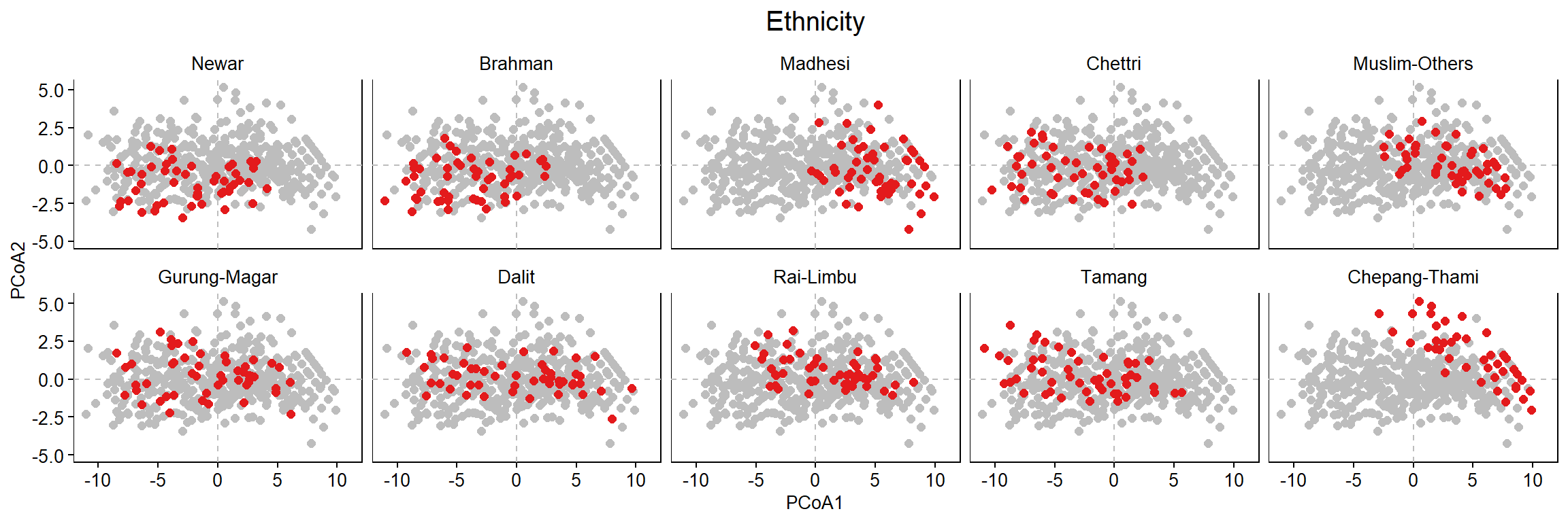
Fit FuelType factors onto the ordination
set.seed(12345)
efit <- vegan::envfit(ord=bd_eth, env=df[,5:10], permutations=1000, strata=NULL, choices=c(1,2), display="sites")

dfit <- data.frame(Category=rownames(efit$vectors$arrows), efit$vectors$arrows[,1:2])
dfit$Category <- factor(dfit$Category, levels=dfit$Category)
Get Centroids: Ethnicity
# Get Centroids
df_eth <- data.frame(Category=rownames(bd_eth$centroids[,1:2]), bd_eth$centroids[,1:2])
df_eth$Category <- as.character(df_eth$Category)

#Factorize ---
df_eth$Category <- factor(df_eth$Category, levels=type_eth)
Plot Ordination Centroids: Ethnicity
# PLOT ---
p12 <- ggplot(df_eth, aes(x=PCoA1, y=PCoA2, label=Category)) +
        geom_hline(yintercept=0, linetype="dashed", color = "#bdbdbd") +
        geom_vline(xintercept=0, linetype="dashed", color = "#bdbdbd") +
        geom_point(aes(fill=Category, color=Category), size=5, shape=16) +
        scale_color_manual(values=cpalette.eth) +
        geom_text(size=3, hjust=0, nudge_x=-0.5, nudge_y=-0.1) +
        geom_text(data=dfit, aes(x=PCoA1, y=PCoA2, label=Category), size = 3, vjust=1, color="red") +
        geom_segment(data=dfit, aes(x=0, y=0, xend=PCoA1, yend=PCoA2, label=Category),
                     arrow=arrow(length=unit(0.2,"cm")), alpha=0.75, color="red") +
        coord_cartesian(xlim=c(-6, 6)) +
        theme(
          axis.text.x = element_text(size = 10, color="#000000"),
          axis.text.y = element_text(size = 10, color="#000000"),
          axis.title = element_text(size = 10, color="#000000"),
          plot.title = element_text(size = 15, color="#000000", hjust=0.5),
          panel.grid.major = element_blank(),
          panel.grid.minor = element_blank(),
          axis.ticks = element_line(size=0.4, color="#000000"),
          strip.text = element_text(size=10, color="#000000"),
          strip.background = element_rect(fill="#FFFFFF", color="#FFFFFF"),
          panel.background = element_rect(fill="#FFFFFF", color="#000000"),
          legend.text = element_text(size = 10, color="#000000"),
          legend.title = element_blank(),
          legend.key.size = unit(0.5, "cm"),
          legend.position = "right") +
      ylab("PCoA2") +
      xlab("PCoA1") +
      ggtitle("Centroids: Ethnicity")
## Warning: Ignoring unknown aesthetics: labelp12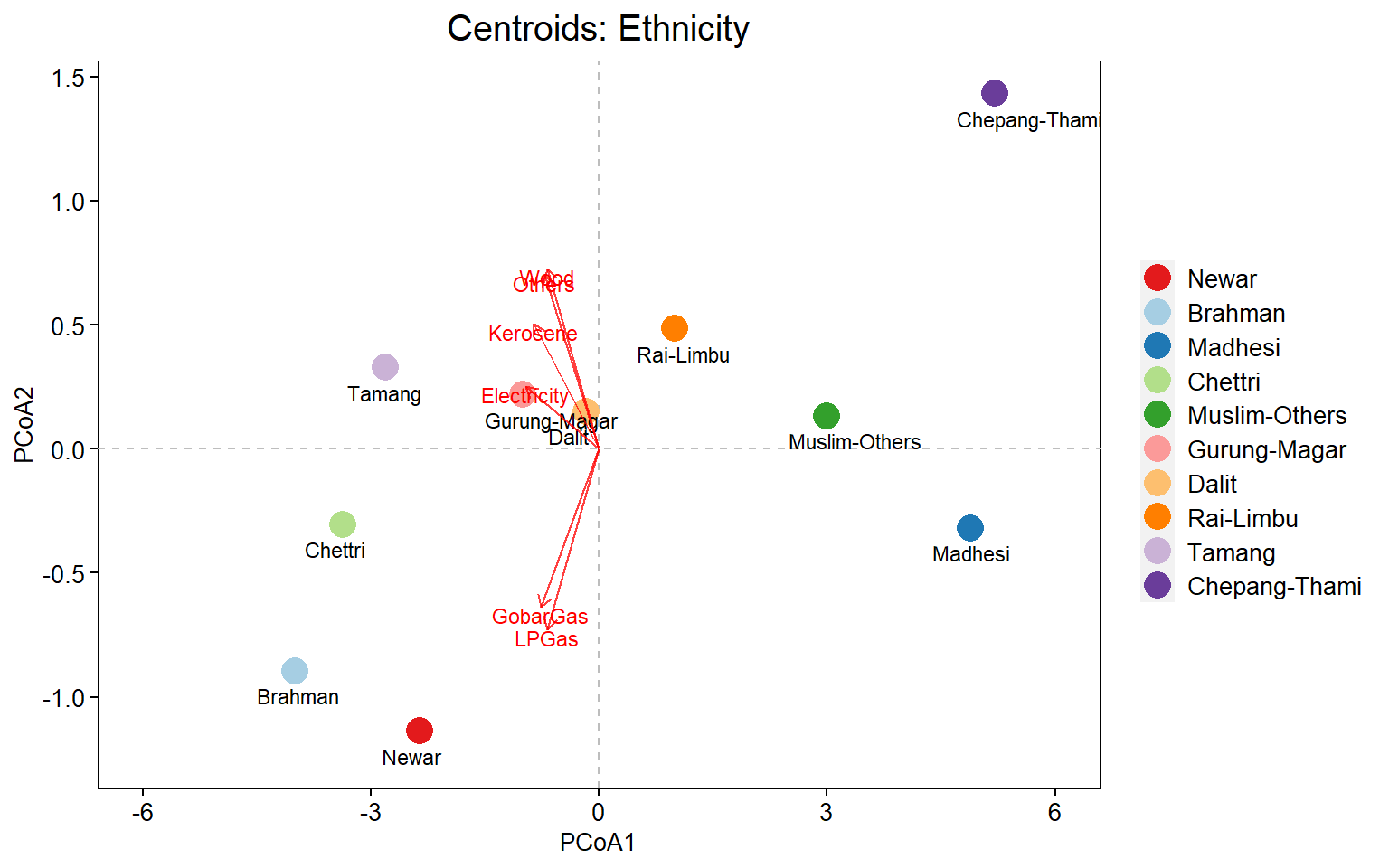
B. Ordination: by IncomeGroup
# BETA DIVERSITY ---
bd_inc <- vegan::betadisper(d=dm, group=df$IncomeGroup, type="centroid")

bd_inc
##
## Homogeneity of multivariate dispersions
##
## Call: vegan::betadisper(d = dm, group = df$IncomeGroup, type =
## "centroid")
##
## No. of Positive Eigenvalues: 6
## No. of Negative Eigenvalues: 0
##
## Average distance to centroid:
## 0-10000 10000-20000 20000-30000 30000-50000 50000-ABOVE
## 4.969 4.560 4.179 3.812 3.317
##
## Eigenvalues for PCoA axes:
## PCoA1 PCoA2 PCoA3 PCoA4 PCoA5 PCoA6
## 11684.2 1048.3 847.6 436.9 159.2 139.1# GET EIGENVALUES ---
d_inc <- data.frame(IncomeGroup=df$IncomeGroup, bd_inc$vectors[,1:2])
d_inc$IncomeGroup <- factor(d_inc$IncomeGroup, levels=type_inc)Plot Ordination
# PLOT ---
p2 <- ggplot(d_inc, aes(x=PCoA1, y=PCoA2)) +
          geom_hline(yintercept=0, linetype="dashed", color = "#bdbdbd") +
          geom_vline(xintercept=0, linetype="dashed", color = "#bdbdbd") +
          geom_point(aes(fill=IncomeGroup, color=IncomeGroup), size=3, shape=18) +
          scale_color_manual(values=cpalette.inc) +
          coord_cartesian(xlim=c(-11, 11), ylim=c(-5,5.2)) +
          theme(
               axis.text.x = element_text(size = 10, color="#000000"),
               axis.text.y = element_text(size = 10, color="#000000"),
               axis.title = element_text(size = 10, color="#000000"),
               plot.title = element_text(size = 15, color="#000000", hjust=0.5),
               panel.grid.major = element_blank(),
               panel.grid.minor = element_blank(),
               axis.ticks = element_line(size=0.4, color="#000000"),
               strip.text = element_text(size=10, color="#000000"),
               strip.background = element_rect(fill="#FFFFFF", color="#FFFFFF"),
               panel.background = element_rect(fill="#FFFFFF", color="#000000"),
               legend.text = element_text(size = 10, color="#000000"),
               legend.title = element_blank(),
               legend.key.size = unit(0.5, "cm"),
               legend.position = "right") +
          ylab("PCoA2") +
          xlab("PCoA1") +
          ggtitle("IncomeGroup")

p2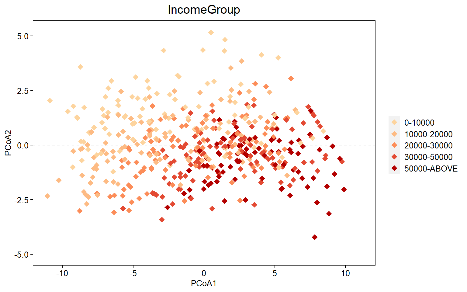
Prepare data for Segregated Plot by IncomeGroup
# PREPARE DATA ---
list.dt <- list()
for(k in 1:length(type_inc)){
  d <- d_inc
  d$Label <- "bg"
  d$Group <- type_inc[k]
  ind <- which(str_detect(as.character(d$IncomeGroup), type_inc[k]) == TRUE)
  d$Label[ind] <- "fg"
  d <- d[order(d$Label, decreasing = FALSE),]
  list.dt[[k]] <- d
}

# AGGREGATE DATA ---
dt <- do.call(rbind.data.frame, list.dt)

# FACTORIZE ---
dt$IncomeGroup <- factor(dt$IncomeGroup, levels=type_inc)
dt$Group <- factor(dt$Group, levels=type_inc)
dt$Label <- factor(dt$Label, levels=c("fg","bg"))
Plot Ordination
# PLOT ---
p21 <- ggplot(dt, aes(x=PCoA1, y=PCoA2)) +
          geom_hline(yintercept=0, linetype="dashed", color = "#bdbdbd") +
          geom_vline(xintercept=0, linetype="dashed", color = "#bdbdbd") +
          geom_point(aes(fill=Label, color=Label), size=2, shape=18) +
          scale_color_manual(values=cpalette.grp) +
          coord_cartesian(xlim=c(-11, 11), ylim=c(-5,5.2)) +
          facet_wrap(~Group, ncol=5, scales="fixed", drop=FALSE, strip.position="top") +
          theme(
               axis.text.x = element_text(size = 10, color="#000000"),
               axis.text.y = element_text(size = 10, color="#000000"),
               axis.title = element_text(size = 10, color="#000000"),
               plot.title = element_text(size = 15, color="#000000", hjust=0.5),
               panel.grid.major = element_blank(),
               panel.grid.minor = element_blank(),
               axis.ticks = element_line(size=0.4, color="#000000"),
               strip.text = element_text(size=10, color="#000000"),
               strip.background = element_rect(fill="#FFFFFF", color="#FFFFFF"),
               panel.background = element_rect(fill="#FFFFFF", color="#000000"),
               legend.text = element_text(size = 10, color="#000000"),
               legend.title = element_blank(),
               legend.key.size = unit(0.5, "cm"),
               legend.position = "none") +
          ylab("PCoA2") +
          xlab("PCoA1") +
          ggtitle("IncomeGroup")

p21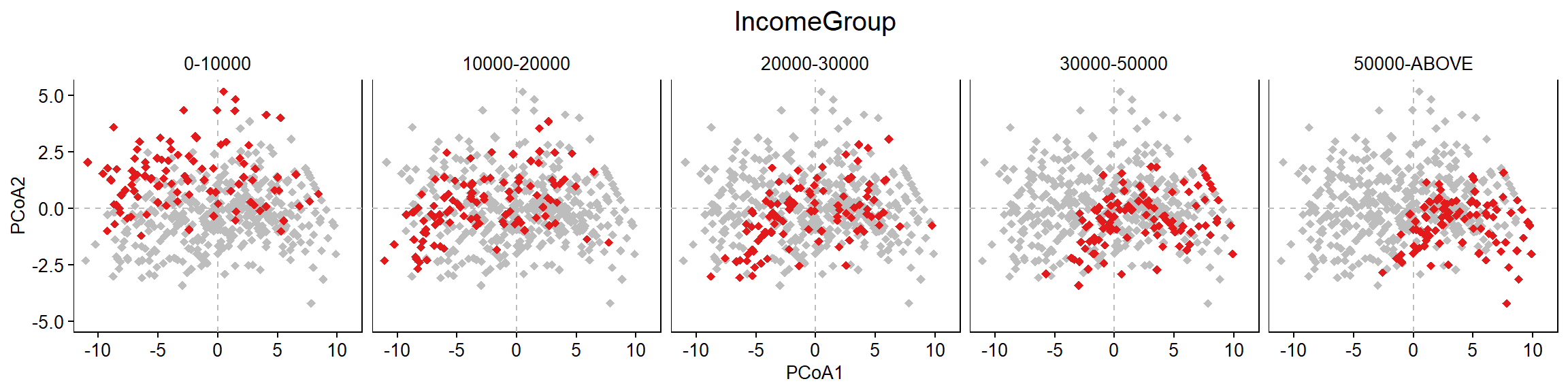
Get Centroids: IncomeGroup
# Get Centroids
df_inc <- data.frame(Category=rownames(bd_inc$centroids[,1:2]), bd_inc$centroids[,1:2])
df_inc$Category <- as.character(df_inc$Category)

#Factorize ---
df_inc$Category <- factor(df_inc$Category, levels=type_inc)
Plot Ordination Centroids: IncomeGroup
# PLOT ---
p22 <- ggplot(df_inc, aes(x=PCoA1, y=PCoA2, label=Category)) +
        geom_hline(yintercept=0, linetype="dashed", color = "#bdbdbd") +
        geom_vline(xintercept=0, linetype="dashed", color = "#bdbdbd") +
        geom_point(aes(fill=Category, color=Category), size=5, shape=16) +
        scale_color_manual(values=cpalette.inc) +
        geom_text(size=3, hjust=0, nudge_x=-0.5, nudge_y=-0.1) +
        coord_cartesian(xlim=c(-6, 6)) +
        theme(
          axis.text.x = element_text(size = 10, color="#000000"),
          axis.text.y = element_text(size = 10, color="#000000"),
          axis.title = element_text(size = 10, color="#000000"),
          plot.title = element_text(size = 15, color="#000000", hjust=0.5),
          panel.grid.major = element_blank(),
          panel.grid.minor = element_blank(),
          axis.ticks = element_line(size=0.4, color="#000000"),
          strip.text = element_text(size=10, color="#000000"),
          strip.background = element_rect(fill="#FFFFFF", color="#FFFFFF"),
          panel.background = element_rect(fill="#FFFFFF", color="#000000"),
          legend.text = element_text(size = 10, color="#000000"),
          legend.title = element_blank(),
          legend.key.size = unit(0.5, "cm"),
          legend.position = "right") +
      ylab("PCoA2") +
      xlab("PCoA1") +
      ggtitle("Centroids: IncomeGroup")

p22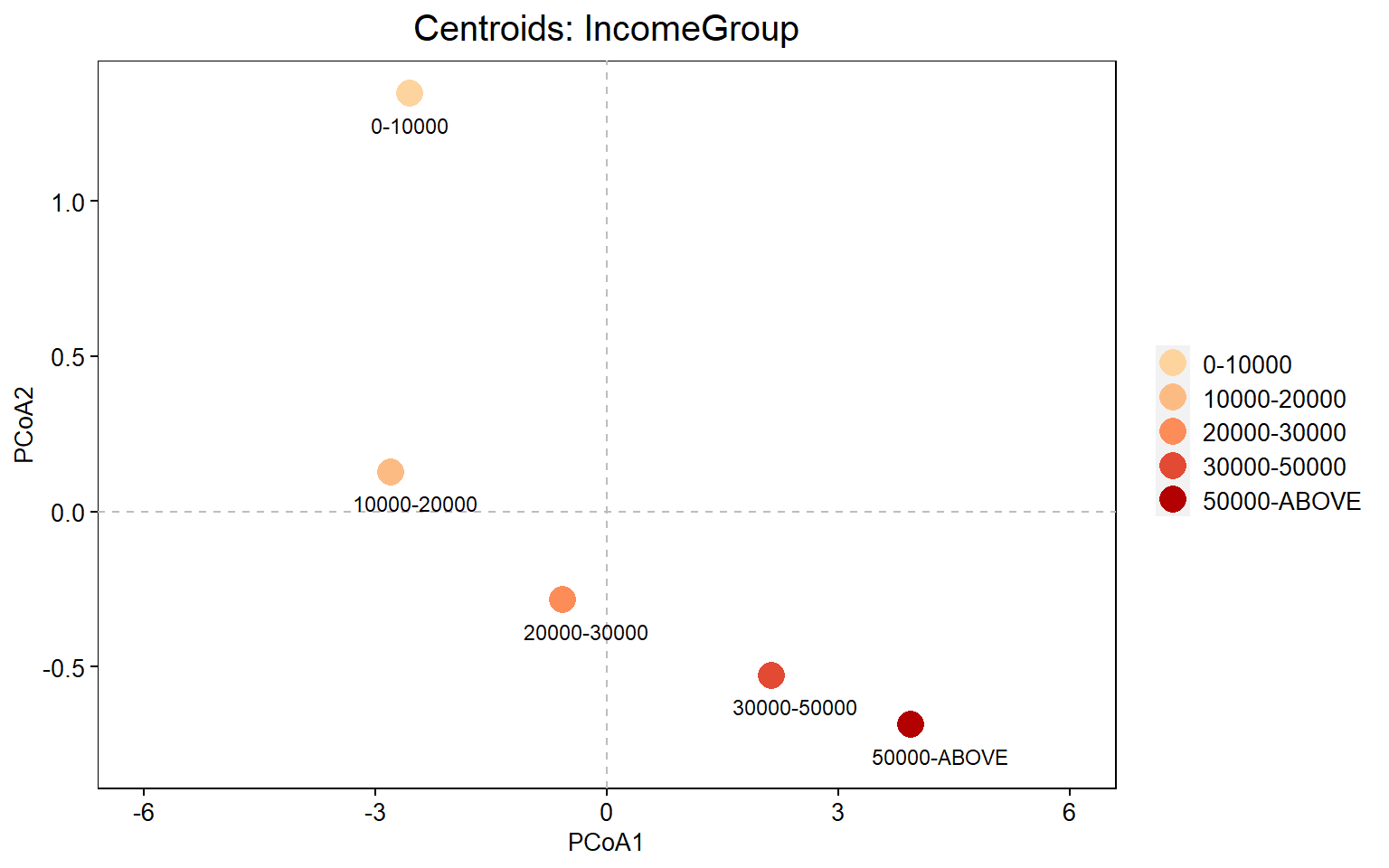
C. Ordination: by EducationLevel
# BETA DIVERSITY ---
bd_edu <- vegan::betadisper(d=dm, group=df$EducationLevel, type="centroid")

bd_edu
##
## Homogeneity of multivariate dispersions
##
## Call: vegan::betadisper(d = dm, group = df$EducationLevel, type =
## "centroid")
##
## No. of Positive Eigenvalues: 6
## No. of Negative Eigenvalues: 0
##
## Average distance to centroid:
## Illiterate NonFormal-Other Primary Secondary University
## 4.802 4.562 4.690 4.781 3.547
##
## Eigenvalues for PCoA axes:
## PCoA1 PCoA2 PCoA3 PCoA4 PCoA5 PCoA6
## 11684.2 1048.3 847.6 436.9 159.2 139.1# GET EIGENVALUES ---
d_edu <- data.frame(EducationLevel=df$EducationLevel, bd_edu$vectors[,1:2])
d_edu$EducationLevel <- factor(d_edu$EducationLevel, levels=type_edu)Plot Ordination
# PLOT ---
p3 <- ggplot(d_edu, aes(x=PCoA1, y=PCoA2)) +
          geom_hline(yintercept=0, linetype="dashed", color = "#bdbdbd") +
          geom_vline(xintercept=0, linetype="dashed", color = "#bdbdbd") +
          geom_point(aes(fill=EducationLevel, color=EducationLevel), size=3, shape=17) +
          scale_color_manual(values=cpalette.edu) +
          coord_cartesian(xlim=c(-11, 11), ylim=c(-5,5.2)) +
          theme(
               axis.text.x = element_text(size = 10, color="#000000"),
               axis.text.y = element_text(size = 10, color="#000000"),
               axis.title = element_text(size = 10, color="#000000"),
               plot.title = element_text(size = 15, color="#000000", hjust=0.5),
               panel.grid.major = element_blank(),
               panel.grid.minor = element_blank(),
               axis.ticks = element_line(size=0.4, color="#000000"),
               strip.text = element_text(size=10, color="#000000"),
               strip.background = element_rect(fill="#FFFFFF", color="#FFFFFF"),
               panel.background = element_rect(fill="#FFFFFF", color="#000000"),
               legend.text = element_text(size = 10, color="#000000"),
               legend.title = element_blank(),
               legend.key.size = unit(0.5, "cm"),
               legend.position = "right") +
          ylab("PCoA2") +
          xlab("PCoA1") +
          ggtitle("EducationLevel")

p3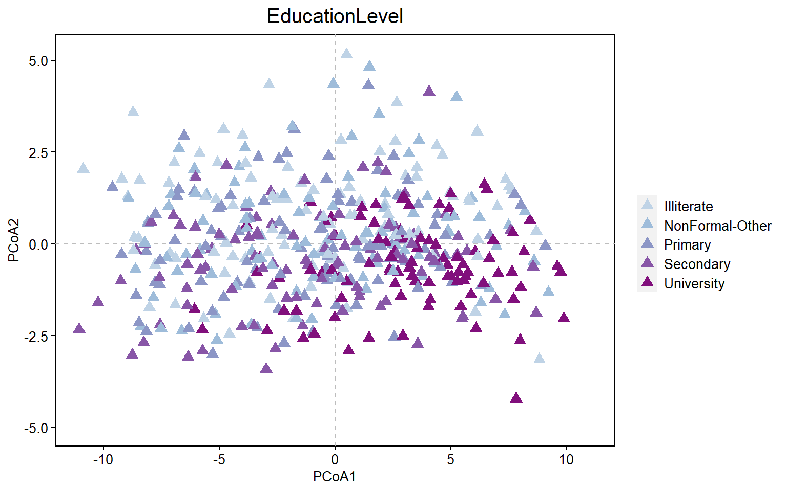
Prepare data for Segregated Plot by EducationLevel
# PREPARE DATA ---
list.dt <- list()
for(k in 1:length(type_edu)){
  d <- d_edu
  d$Label <- "bg"
  d$Group <- type_edu[k]
  ind <- which(str_detect(as.character(d$EducationLevel), type_edu[k]) == TRUE)
  d$Label[ind] <- "fg"
  d <- d[order(d$Label, decreasing = FALSE),]
  list.dt[[k]] <- d
}

# AGGREGATE DATA ---
dt <- do.call(rbind.data.frame, list.dt)

# FACTORIZE ---
dt$EducationLevel <- factor(dt$EducationLevel, levels=type_edu)
dt$Group <- factor(dt$Group, levels=type_edu)
dt$Label <- factor(dt$Label, levels=c("fg","bg"))
Plot Ordination
# PLOT ---
p31 <- ggplot(dt, aes(x=PCoA1, y=PCoA2)) +
          geom_hline(yintercept=0, linetype="dashed", color = "#bdbdbd") +
          geom_vline(xintercept=0, linetype="dashed", color = "#bdbdbd") +
          geom_point(aes(fill=Label, color=Label), size=2, shape=17) +
          scale_color_manual(values=cpalette.grp) +
          coord_cartesian(xlim=c(-11, 11), ylim=c(-5,5.2)) +
          facet_wrap(~Group, ncol=5, scales="fixed", drop=FALSE, strip.position="top") +
          theme(
               axis.text.x = element_text(size = 10, color="#000000"),
               axis.text.y = element_text(size = 10, color="#000000"),
               axis.title = element_text(size = 10, color="#000000"),
               plot.title = element_text(size = 15, color="#000000", hjust=0.5),
               panel.grid.major = element_blank(),
               panel.grid.minor = element_blank(),
               axis.ticks = element_line(size=0.4, color="#000000"),
               strip.text = element_text(size=10, color="#000000"),
               strip.background = element_rect(fill="#FFFFFF", color="#FFFFFF"),
               panel.background = element_rect(fill="#FFFFFF", color="#000000"),
               legend.text = element_text(size = 10, color="#000000"),
               legend.title = element_blank(),
               legend.key.size = unit(0.5, "cm"),
               legend.position = "none") +
          ylab("PCoA2") +
          xlab("PCoA1") +
          ggtitle("EducationLevel")

p31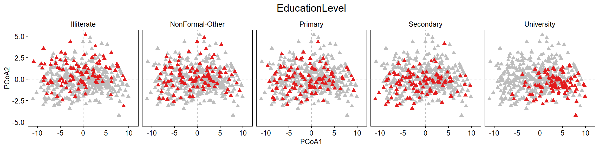
Get Centroids: EducationLevel
# Get Centroids
df_edu <- data.frame(Category=rownames(bd_edu$centroids[,1:2]), bd_edu$centroids[,1:2])
df_edu$Category <- as.character(df_edu$Category)

#Factorize ---
df_edu$Category <- factor(df_edu$Category, levels=type_edu)
Plot Ordination Centroids: EducationLevel
# PLOT ---
p32 <- ggplot(df_edu, aes(x=PCoA1, y=PCoA2, label=Category)) +
        geom_hline(yintercept=0, linetype="dashed", color = "#bdbdbd") +
        geom_vline(xintercept=0, linetype="dashed", color = "#bdbdbd") +
        geom_point(aes(fill=Category, color=Category), size=5, shape=16) +
        scale_color_manual(values=cpalette.edu) +
        geom_text(size=3, hjust=0, nudge_x=-0.5, nudge_y=-0.1) +
        coord_cartesian(xlim=c(-6, 6)) +
        theme(
          axis.text.x = element_text(size = 10, color="#000000"),
          axis.text.y = element_text(size = 10, color="#000000"),
          axis.title = element_text(size = 10, color="#000000"),
          plot.title = element_text(size = 15, color="#000000", hjust=0.5),
          panel.grid.major = element_blank(),
          panel.grid.minor = element_blank(),
          axis.ticks = element_line(size=0.4, color="#000000"),
          strip.text = element_text(size=10, color="#000000"),
          strip.background = element_rect(fill="#FFFFFF", color="#FFFFFF"),
          panel.background = element_rect(fill="#FFFFFF", color="#000000"),
          legend.text = element_text(size = 10, color="#000000"),
          legend.title = element_blank(),
          legend.key.size = unit(0.5, "cm"),
          legend.position = "right") +
      ylab("PCoA2") +
      xlab("PCoA1") +
      ggtitle("Centroids: EducationLevel")

p32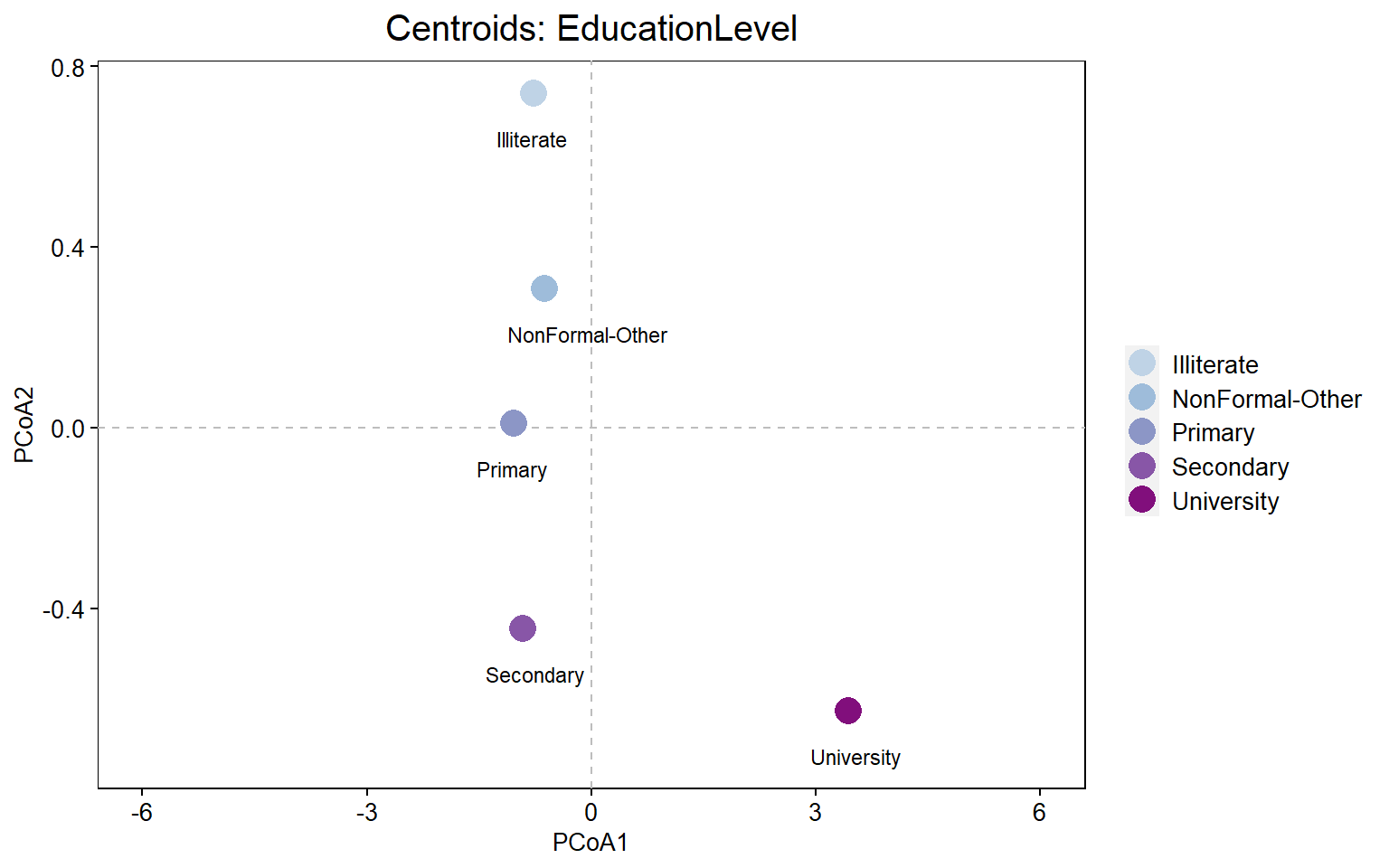
D. Ordination: by GeoRegion
# BETA DIVERSITY ---
bd_geo <- vegan::betadisper(d=dm, group=df$GeoRegion, type="centroid")

bd_geo
##
## Homogeneity of multivariate dispersions
##
## Call: vegan::betadisper(d = dm, group = df$GeoRegion, type =
## "centroid")
##
## No. of Positive Eigenvalues: 6
## No. of Negative Eigenvalues: 0
##
## Average distance to centroid:
## Himalayan Hilly
## 4.386 4.973
##
## Eigenvalues for PCoA axes:
## PCoA1 PCoA2 PCoA3 PCoA4 PCoA5 PCoA6
## 11684.2 1048.3 847.6 436.9 159.2 139.1# GET EIGENVALUES ---
d_geo <- data.frame(GeoRegion=df$GeoRegion, bd_geo$vectors[,1:2])
d_geo$GeoRegion <- factor(d_geo$GeoRegion, levels=type_geo)Plot Ordination
# PLOT ---
p4 <- ggplot(d_geo, aes(x=PCoA1, y=PCoA2)) +
          geom_hline(yintercept=0, linetype="dashed", color = "#bdbdbd") +
          geom_vline(xintercept=0, linetype="dashed", color = "#bdbdbd") +
          geom_point(aes(fill=GeoRegion, color=GeoRegion), size=3, shape=15) +
          scale_color_manual(values=cpalette.geo) +
          coord_cartesian(xlim=c(-11, 11), ylim=c(-5,5.2)) +
          theme(
               axis.text.x = element_text(size = 10, color="#000000"),
               axis.text.y = element_text(size = 10, color="#000000"),
               axis.title = element_text(size = 10, color="#000000"),
               plot.title = element_text(size = 15, color="#000000", hjust=0.5),
               panel.grid.major = element_blank(),
               panel.grid.minor = element_blank(),
               axis.ticks = element_line(size=0.4, color="#000000"),
               strip.text = element_text(size=10, color="#000000"),
               strip.background = element_rect(fill="#FFFFFF", color="#FFFFFF"),
               panel.background = element_rect(fill="#FFFFFF", color="#000000"),
               legend.text = element_text(size = 10, color="#000000"),
               legend.title = element_blank(),
               legend.key.size = unit(0.5, "cm"),
               legend.position = "right") +
          ylab("PCoA2") +
          xlab("PCoA1") +
          ggtitle("GeoRegion")

p4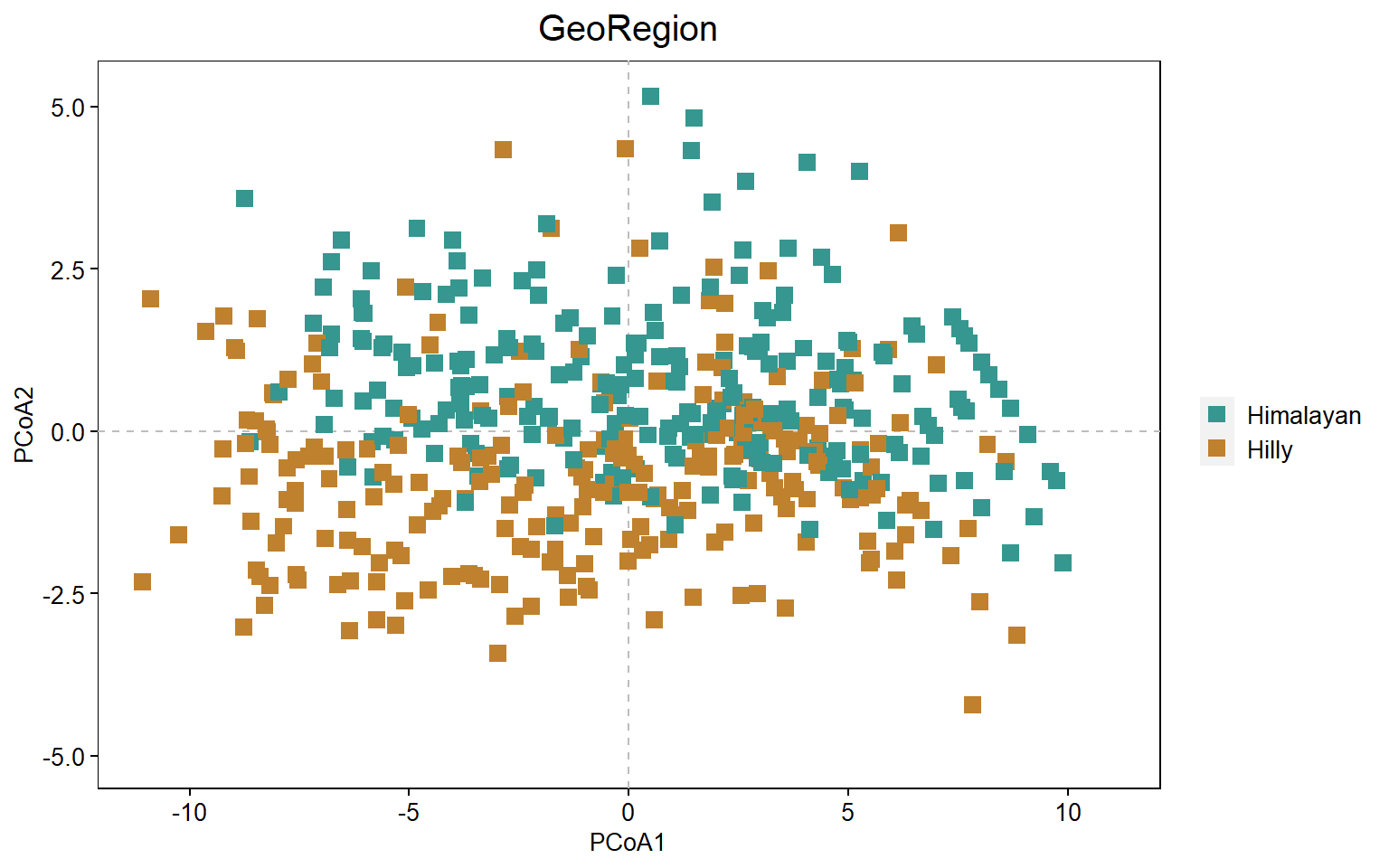
Prepare data for Segregated Plot by GeoRegion
# PREPARE DATA ---
list.dt <- list()
for(k in 1:length(type_geo)){
  d <- d_geo
  d$Label <- "bg"
  d$Group <- type_geo[k]
  ind <- which(str_detect(as.character(d$GeoRegion), type_geo[k]) == TRUE)
  d$Label[ind] <- "fg"
  d <- d[order(d$Label, decreasing = FALSE),]
  list.dt[[k]] <- d
}

# AGGREGATE DATA ---
dt <- do.call(rbind.data.frame, list.dt)

# FACTORIZE ---
dt$GeoRegion <- factor(dt$GeoRegion, levels=type_geo)
dt$Group <- factor(dt$Group, levels=type_geo)
dt$Label <- factor(dt$Label, levels=c("fg","bg"))
Plot Ordination
# PLOT ---
p41 <- ggplot(dt, aes(x=PCoA1, y=PCoA2)) +
          geom_hline(yintercept=0, linetype="dashed", color = "#bdbdbd") +
          geom_vline(xintercept=0, linetype="dashed", color = "#bdbdbd") +
          geom_point(aes(fill=Label, color=Label), size=2, shape=15) +
          scale_color_manual(values=cpalette.grp) +
          coord_cartesian(xlim=c(-11, 11), ylim=c(-5,5.2)) +
          facet_wrap(~Group, ncol=5, scales="fixed", drop=FALSE, strip.position="top") +
          theme(
               axis.text.x = element_text(size = 10, color="#000000"),
               axis.text.y = element_text(size = 10, color="#000000"),
               axis.title = element_text(size = 10, color="#000000"),
               plot.title = element_text(size = 15, color="#000000", hjust=0.5),
               panel.grid.major = element_blank(),
               panel.grid.minor = element_blank(),
               axis.ticks = element_line(size=0.4, color="#000000"),
               strip.text = element_text(size=10, color="#000000"),
               strip.background = element_rect(fill="#FFFFFF", color="#FFFFFF"),
               panel.background = element_rect(fill="#FFFFFF", color="#000000"),
               legend.text = element_text(size = 10, color="#000000"),
               legend.title = element_blank(),
               legend.key.size = unit(0.5, "cm"),
               legend.position = "none") +
          ylab("PCoA2") +
          xlab("PCoA1") +
          ggtitle("GeoRegion")

p41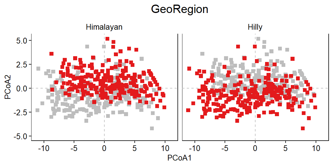
Get Centroids: GeoRegion
# Get Centroids
df_geo <- data.frame(Category=rownames(bd_geo$centroids[,1:2]), bd_geo$centroids[,1:2])
df_geo$Category <- as.character(df_geo$Category)

#Factorize ---
df_geo$Category <- factor(df_geo$Category, levels=type_geo)
Plot Ordination Centroids: GeoRegion
# PLOT ---
p42 <- ggplot(df_geo, aes(x=PCoA1, y=PCoA2, label=Category)) +
        geom_hline(yintercept=0, linetype="dashed", color = "#bdbdbd") +
        geom_vline(xintercept=0, linetype="dashed", color = "#bdbdbd") +
        geom_point(aes(fill=Category, color=Category), size=5, shape=16) +
        scale_color_manual(values=cpalette.geo) +
        geom_text(size=3, hjust=0, nudge_x=-0.5, nudge_y=-0.1) +
        coord_cartesian(xlim=c(-6, 6)) +
        theme(
          axis.text.x = element_text(size = 10, color="#000000"),
          axis.text.y = element_text(size = 10, color="#000000"),
          axis.title = element_text(size = 10, color="#000000"),
          plot.title = element_text(size = 15, color="#000000", hjust=0.5),
          panel.grid.major = element_blank(),
          panel.grid.minor = element_blank(),
          axis.ticks = element_line(size=0.4, color="#000000"),
          strip.text = element_text(size=10, color="#000000"),
          strip.background = element_rect(fill="#FFFFFF", color="#FFFFFF"),
          panel.background = element_rect(fill="#FFFFFF", color="#000000"),
          legend.text = element_text(size = 10, color="#000000"),
          legend.title = element_blank(),
          legend.key.size = unit(0.5, "cm"),
          legend.position = "right") +
      ylab("PCoA2") +
      xlab("PCoA1") +
      ggtitle("Centroids: GeoRegion")

p42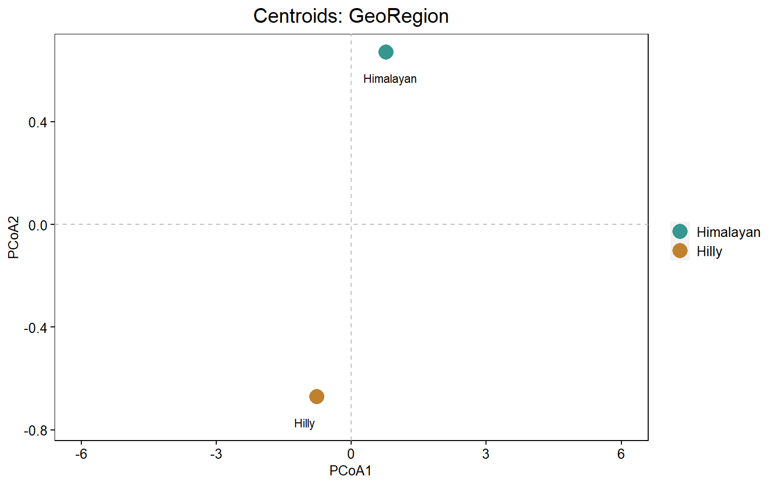
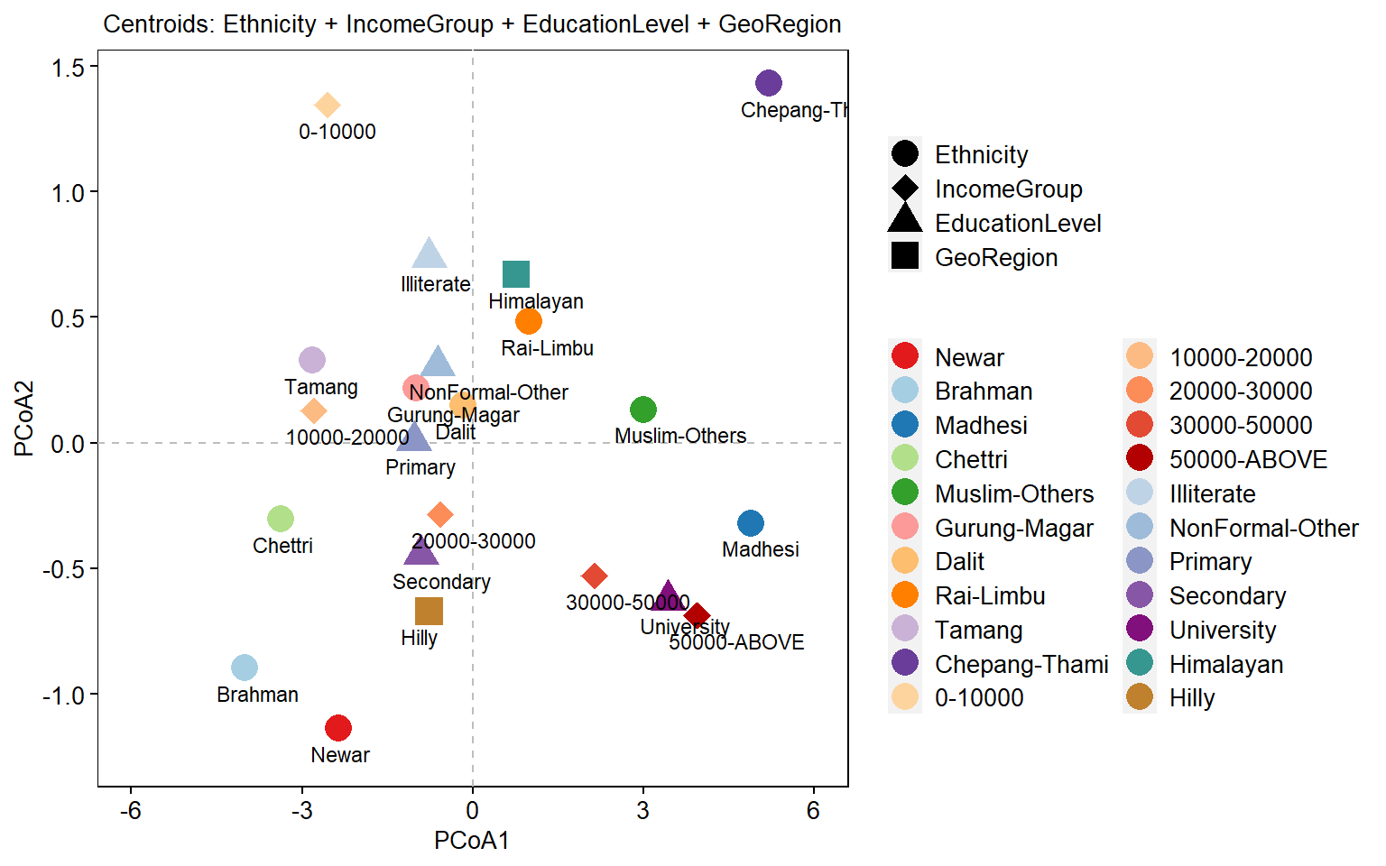
E. Merge Centroid Data: Ethnicity + IncomeGroup + EducationLevel + GeoRegion
df_eth$Group <- "Ethnicity"
df_inc$Group <- "IncomeGroup"
df_edu$Group <- "EducationLevel"
df_geo$Group <- "GeoRegion"
df <- rbind(df_eth, df_inc, df_edu, df_geo)

# FACTORIZE ---
df$Category <- factor(df$Category, levels=c(type_eth, type_inc, type_edu, type_geo))
df$Group <- factor(df$Group, levels=c("Ethnicity","IncomeGroup","EducationLevel","GeoRegion"))
Plot Ordination Centroids: Ethnicity + IncomeGroup + EducationLevel + GeoRegion
# Define Colors ---
jColFun <- colorRampPalette(brewer.pal(n = 9, "Set1"))
cpalette <- c(cpalette.eth, cpalette.inc, cpalette.edu, cpalette.geo)

# PLOT ---
p <- ggplot(df, aes(x=PCoA1, y=PCoA2, label=Category)) +
        geom_hline(yintercept=0, linetype="dashed", color = "#bdbdbd") +
        geom_vline(xintercept=0, linetype="dashed", color = "#bdbdbd") +
        geom_point(aes(fill=Category, color=Category, shape=Group), size=5) +
        scale_color_manual(values=cpalette) +
        scale_shape_manual(values=c(16,18,17,15)) +
        geom_text(size=3, hjust=0, nudge_x=-0.5, nudge_y=-0.1) +
        coord_cartesian(xlim=c(-6, 6)) +
        theme(
          axis.text.x = element_text(size = 10, color="#000000"),
          axis.text.y = element_text(size = 10, color="#000000"),
          axis.title = element_text(size = 10, color="#000000"),
          plot.title = element_text(size = 10, color="#000000", hjust=0.5),
          panel.grid.major = element_blank(),
          panel.grid.minor = element_blank(),
          axis.ticks = element_line(size=0.4, color="#000000"),
          strip.text = element_text(size=10, color="#000000"),
          strip.background = element_rect(fill="#FFFFFF", color="#FFFFFF"),
          panel.background = element_rect(fill="#FFFFFF", color="#000000"),
          legend.text = element_text(size = 10, color="#000000"),
          legend.title = element_blank(),
          legend.key.size = unit(0.5, "cm"),
          legend.position = "right") +
      ylab("PCoA2") +
      xlab("PCoA1") +
      ggtitle("Centroids: Ethnicity + IncomeGroup + EducationLevel + GeoRegion")

p